Introduction to Game-Theoretic Probability
March 19, 2022
\[\newcommand{\R}{\mathbb{R}} \newcommand{\strat}{\varphi} \newcommand{\cp}{\mathcal{K}} \newcommand{\cps}{\cp^\strat} \newcommand{\eps}{\epsilon} \renewcommand{\by}{\bar{y}} \newcommand{\hstrat}{\hat{\strat}} \newcommand{\inf}{\infty}\]- 1. Prelude: A Brief History
- 2. The Setup
- 3. Forcing and Weak Forcing
- 4. Averaging Strategies: The Infinite Casino
- 5. Proving the Game-theoretic LLN
- 6. Resources
1. Prelude: A Brief History
Classical probability emerged largely from thinking about betting and games of chance (e.g., dice and coin tossing), and relied mostly on frequencies and combinatorics for its arguments. While modern probability theory is based on measure theory and Kolmogorov’s axioms, it is still common to teach elementary probabilistic principles using discrete games. For instance, when learning about the law of large numbers, I remember one teacher explaining it as follows: If you flip an unbiased coin and bet on an average outcome other than 1/2, then you will go broke as the coin continues to be flipped.
The analogy runs deeper, however. In his 1939 doctoral thesis Étude Critique de la Notion de Collectif, Jean Ville proved a result which formally ties modern probability to betting (although I don’t believe he knew it yet). Informally it says that, if an event is very unlikely, then there exists a supermartingale which tends to infinity on that event. This is intimately tied to betting because supermartingales represent betting strategies. An “almost sure” event in modern probability thus becomes, in game-theoretic probability, an event for which there exists a betting strategy which would make us infinitely rich if it didn’t come to pass.
More broadly, game-theoretic probability is the formal approach to probability based on games and betting instead of \(\sigma\) algebras and measures. There has been development of these ideas from several perspectives, such as probability, statistical inference, and online learning (see the appendix of this paper for an interesting history and a cool diagram), but has perhaps been most popularized by Glenn Shafer and Vladimir Vovk in their textbook Game-Theoretic Foundations for Probability and Finance.
When introducing an alternative foundation for a subject, a natural question is whether it’s more general. Is the reach of the game-theoretic perspective fundamentally greater than the Kolmogorov axioms; the results of the former a superset of the latter? The answer is … sort of? Modern and game-theoretic probability are equivalent for some games we’ll consider. After that, as Shafer and Vovk say in their book, they generalize these core examples in different directions. But then they also go onto say that they can connect them more systemically by means of martingales. So I’m not actually sure anyone knows precisely whether one formalization is strictly more powerful than the other. What is certain though, is that you can improve on measure-theoretic results by using game-theoretic probability and translating the results into measure-theory by means of martingales. Again, see this recent paper as an example. For that reason alone, understanding game-theoretic probability is valuable.
2. The Setup
Consider a full information game between three players: Alice, Bob, and World. It proceeds as follows:
- Bob has some initial capital, \(C_0\).
- For rounds \(n=1,2,\dots\)
- Alice announces a value \(v_n\)
- Bob announces a value \(M_n\)
- World announces \(y_n\in[-B,B]\)
- Bob’s new capital is \(C_n = C_{n-1} + M_n(y_n - v_n)\)
It’s helpful to consider yourself as playing Bob, and against Alice and World (who we’ll henceforth call the opponents). Naturally, you want to become rich as play progresses, i.e.,
\[C_n \xrightarrow{n\to\infty} \infty,\]or, barring that, you want to constrain the behavior of Alice and World – that is, to force them to play particular values. Basically, if we can’t get our way and become infinitely wealthy, let’s be sure to exact some vengeance. For example, in the game above one can show that you can force them to agree with each other in the limit:
\[\begin{equation} \label{eq:lln_general} \lim_{n\to\infty} \frac{1}{n}\sum_{i=1}^n (y_i - v_i) = 0. \tag{1} \end{equation}\]In the language of game-theoretic probability, \(M_n\) is the bet that Bob is placing on the forecast \(v_n\). If \(M>0\), he’s assuming \(y_n\) will be greater than \(v_n\). Likewise for \(M_n<0\). If his bet is correct, he’ll add \(\vert M_n(y_n-v_n)\vert\) to his capital; otherwise he loses the same amount.
Essentially, game-theoretic probability is the study of what can be achieved by Bob in various kinds of games. The simplified game in which Alice always announces the same value – zero – results in the game-theoretic law of large numbers:
- Bob has some initial capital, \(C_0\).
- For rounds \(n=1,2,\dots\)
- Bob annonces a value \(M_n\)
- World announces \(y_n\in[-B,B]\)
- Bob’s new capital is \(S\) is \(C_n = C_{n-1} + M_ny_n\).
Here we can ensure that either Bob becomes infinitely rich, or
\[\begin{equation} \label{eq:lln} \frac{1}{n}\sum_{i=1}^n y_i \to 0. \tag{2} \end{equation}\]Stare at these games for a second. Notice that we haven’t introduced an underlying probability space, any distributional assumptions on any of the players, or any notions of independence (except arguably for the Alice in the last game). There’s not even any notion of randomness. This is kind of remarkable. Normally, you can’t even begin to get off the ground without rigorously defining these things. Also, because the games are sequential in nature, results achieved in this space are inherently sequential as well.
The rest of the post will focus on the second game and proving Equation \(\eqref{eq:lln}\).
2.1 Some Terminology
To begin rigorously analyzing such games, we need to introduce various concepts.
Like most areas of math, there’s a slew of new (ish?) terminology that goes along with it. Most of it is intuitive and often you can get by without paying too much attention to the precise definitons. But we still need to introduce several precise meanings to start proving things.
An event is a condition on the opponents. E.g., Equations \(\eqref{eq:lln_general}\) and \(\eqref{eq:lln}\) are events. Let \(\Omega_\inf\) be the set of all infinite move sequences by the opponents, and \(\Omega\) the set of all finite move sequences. E.g., \(\{y_1,v_1,y_2,v_2,\dots\}\in \Omega_\inf\) and \(\{y_1,v_1,\dots,y_n,v_n\}\in\Omega\). Since we’re analyzing the game in which Alice always plays 0, we’ll omit \(v_i\) from these sequences. Formally, we call \(\Omega_\inf\) the sample space, and \(\Omega\) the set of all situations. An event is a subset \(E\subset \Omega_\inf\), and a path is an element \(\omega\in\Omega_\inf\). Typically, it will be clear from context (or not matter) whether we’re talking about finite or infinite sequences so we’ll abuse notation and just write \(\Omega\) for both \(\Omega_\inf\) and \(\Omega\).
Most the results in the space involve constructing strategies for Bob. Formally, a strategy is a pair \((C_0, \strat)\) where \(C_0\) is the initial capital and \(\strat\) is an predictable process, which is a function
\[\strat:\Omega\to\R,\]Given \(\omega\in\Omega_\inf\cup \Omega\) write \(\omega^n\) for the first \(n\) elements of \(\omega\), i.e., the first \(n\) moves by world. To say that \(\strat\) is predictable just means that the functions
\[\strat_n: \Omega_\inf\to\R:\omega \mapsto \strat(\omega^n),\]depend only on \(\omega^{n-1}\). That is, the \(n\)-th move of Bob’s strategy depends only on the first \(n-1\) moves by World.
If any of this is overly confusing, you can probably just ignore it. A path is a sequence of moves by World, and \(\strat\) is a betting strategy for Bob which determines the amount to bet given what’s already happened in the game. The rest is details.
2.2 The Capital Process
Bob’s capital process is a function \(\cps_n(\omega)\) is a function of his strategy \(\omega\), the moves made by World \(\omega\), and tracks how his capital evolves over time. Its definition depends on the exact game being played. For the first game above it is defined recursively as
\[\begin{equation} \cps_n(\omega) = \cps_{n-1}(\omega) + \strat_{n-1}(\omega)( y_{n-1} - v_{n-1}), \end{equation}\]with \(\cps_0=C_0\), the initial capital. For the second game above, and the one we’re analyzing, it is
\[\begin{equation} \label{eq:cp} \cps_n(\omega) = \cps_{n-1}(\omega) + \strat_{n-1}(\omega) y_{n-1}, \tag{3} \end{equation}\]since \(v_n=0\). The dependence on \(\omega\) is usually dropped. Results will involve developing a strategy \(\strat\) such that \(\eqref{eq:cp}\) can be analyzed.
3. Forcing and Weak Forcing
A foundational concept is normal probability is an almost sure event. Here, as alluded to above, this means an event \(E\) such that \(\cps\geq 0\) and either
\[\lim_n \cps =\infty\quad\text{or}\quad E \text{ happens}.\]That is, Bob does not risk bankruptcy and either becomes infinitely rich or forces \(E\) to occur. For this reason, we’ll also say that the Bob can force \(E\). An equivalent way to write this is that for all \(\omega\notin E\), \(\lim_n \cps_n =\infty\).
A strategy \(\strat\) for Bob weakly forces event \(E\) if \(\cp^\strat \geq 0\) and
\[\sup_n \cp^\strat_n(\omega) =\omega\]for all \(\omega\not\in E\).
Weak forcing is (shockingly) a weaker condition than forcing, meaning that meaning that if we can weakly force \(E\) we can force \(E\).
To see that, suppose \(\strat\) is a strategy that weakly forces \(E\), and let \(\omega\notin E\) so that \(\sup_n\cps(\omega)=\infty\). We want to create a strategy \(\hstrat\) such that \(\lim_n \cp^{\hstrat}(\omega)=\infty\) or \(E\) occurs. The idea is to let \(\hstrat\) be a scaled down version of \(\strat\) which sets aside some capital every time \(\cps\) gets large. Since the latter is large infinitely often, we can set aside capital infinitely often, meaning that \(\cp_{\hstrat}\to\infty\).
Let \(\{T_1<T_2<\dots\}\subset\mathbb{N}\), \(i\in\mathbb{N}\) be an infinite increasing sequence of natural numbers. Fix \(0<\beta<1\). Define \(\hstrat\) as playing the same moves as \(\strat\) until \(\cps_n>T_1\). Define the next move \(\hstrat(\omega)\) to bet the amount \(\beta \strat_{n+1}(\omega)\), i.e., a scaled down version of \(\strat\)’s next bet. Thus, if \(\strat\) loses money, \(\hstrat\) loses a little less, and if it wins, \(\hstrat\) wins a little less. Since \(\cps_n\geq 0\), \(\strat\) can lose at most \(\cps_n\), thus \(\hstrat\) can lose at most \(\beta \cp^{\hstrat}_n\), and \((1-\beta) \cp^{\hstrat}_n\) is safe.
Let \(\hstrat\) continuing emulating \(\strat\) until \(\cps_{n}>T_2\), and then repeat the process. Again, we are saving a positive amount of capital which is henceforth saved. This amount builds over time, and since \(\cps\) eventually exceeds \(T_i\) for all \(i\) (otherwise it would be bounded by some finite number), the strategy \(\hstrat\) saves an infinite amount, thus \(\cp^{\hstrat}_n\to\infty.\)
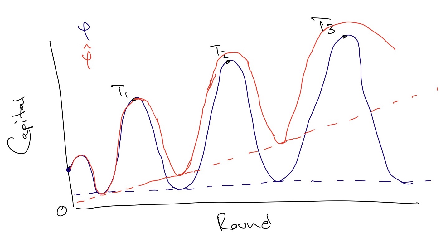
Example of changing strategy \(\strat\) into \(\hstrat\). Here, the capital process of \(\strat\), \(\cps\), has progressively higher peaks, so \(\sup_n \cps_n=\infty\). But it always loses enough capital to return to some baseline value near 0, so that the limit is undefined and in particular, is not infinity. \(\hstrat\) on the other hand, saves capital at thresholds \(T_i\) so that its baseline progressively moves upwards, and is infinite in the limit. In this example, we've selectively chosen \(T_i\) such that they're always at the peaks of \(\cps\) (i.e., \(\strat\) loses the next bet) but this is not necessarily the case. If \(\strat\) wins the bet, \(\hstrat\) simply wins less.
4. Averaging Strategies: The Infinite Casino
Thus far, we’ve conceived of Bob as playing a single game against his opponents. But, as we’ll see, a common technique to force events is to average various strategies. To this end, it’s helpful to consider the Bob as splitting his attention among many games. He walks into an infinite casino with two players, World and Alice, sitting at each table. He can decide to play at any subset of the tables.
Suppose he plays strategy \(\strat_1\) at table 1, and \(\strat_2\) at table 2. We can consider an overall strategy \(\alpha_1\strat_1 + \alpha_2\strat_2\) for any convex combination \(\alpha_1+\alpha_2=1\), and interpret it as Bob splitting his initial capital \(C_0\) between two accounts, putting \(\alpha_1 C_0\) on table 1, and \(\alpha_2 C_0\) on table 2. And there’s no reason he can’t split his capital among infinitely many strategies. In that case, we have the overall strategy
\[\strat = \sum_{i=1}^\infty \alpha_i \strat_i,\]where \(\sum_{i=1}^\infty \alpha_i=1\). For this to be a legitimate strategy, however, we need that \(\sum_i \alpha_i \strat_i\) converges in \(\R\) at each timestep since Bob can only bet a finite amount at any time.
Naturally, the capital process for a strategy \(\sum_i \alpha_i \strat_i\) is
\[\cp_n^{\sum_i \alpha_i \strat_i} = \sum_i \alpha_i \cp_n^{\strat_i}.\]Averaging strategies is useful for the following reason: Suppose \(\strat_1\) forces \(E_1\) and \(\strat_2\) forces \(E_2\). Then \(\strat = \alpha_1\strat_1 + \alpha_2\strat_2\) forces \(E_1\cap E_2\). Seeing this is mostly a matter of unwinding definitions. If \(\omega\) is such that \(\lim_n \cps_n(\omega)<\infty\), then the capital processes of both \(\alpha_1\strat_1\) and \(\alpha_2\strat_2\) are finite as well. But that means, by definition of forcing, that \(E_1\) and \(E_2\) both happen on this path.
This argument can be extended to countably infinite stategies as well. Suppose \(\strat_i\) forces \(E_i\) for \(i=1,2,\dots\). Since \(\cp^{\strat_i}_n=\cp_{n-1}^{\strat_i} + \strat_{i,n}y_n\geq 0\) (by definition of forcing), we have
\[\vert \strat_{i,n} \vert \leq \frac{\cp_{n-1}^{\strat_i}}{B},\]otherwise we could set \(y_n = B\) or \(y_n=-B\) to force bankruptcy. (Here \(\strat_{i,n}\) is the \(n\)-th move of the \(i\)-th strategy.) This, in turn, implies that \(\cp_{i,n}y_n \leq \cp_{n-1}^{\strat_i}\) (since \(y_n\leq B\)). Therefore,
\[\cp_n^{\strat_i}=\cp_{n-1}^{\strat_i} + \strat_{i,n}y_n \leq 2\cp_{n-1}^{\strat_i} = 2(\cp_{n-2}^{\strat_i}+\strat_{i,n-1}y_{n-1})\leq 4\cp_{n-2}^{\strat_i}\leq \dots\leq 2^n C_0.\]Combining this with the inequality above gives
\[\vert \strat_{i,n}\vert \leq \frac{2^n C_0}{B}.\]Consider the strategy
\[\strat = \sum_k 2^{-k} \strat_i,\]which is a valid convex combination because \(\sum_k 2^{-k}=1\), and which converges for fixed \(n\) because
\[\sum_k \vert 2^{-k}\strat_{i,n}\vert \leq \frac{2^nC_0}{B}\sum_k \frac{1}{2^k}=\frac{2^nC_0}{B}<\infty.\]From here, the arguments proceeds the same as above. For a path \(\omega\) with \(\sup_n \cps_n(\omega)<\infty\), it must be the case that \(\sup_n 2^{-k}\cp_n^{\strat_i}<\infty\) as well. Therefore, on this path, \(E_k\) occurs, meaning that \(\cap_{k=1}^\infty E_k\) does too.
5. Proving the Game-theoretic LLN
Recall that our goal is to show that the Bob can force event \(E\) in the second game, where \(E\) is the event
\[\lim_{n\to\infty}\frac{1}{n}\sum_{i=1}^n y_i = 0.\]Put \(\bar{y}_n = \frac{1}{n}\sum_{i=1}^n y_i\). By the arguments above it suffices to show that Bob can weakly force \(E\). To do this, we’ll use a standard approach from analysis. Let \(\eps>0\) and consider the events
\[E^+: \limsup_n \by_n \leq \eps,\quad\text{and}\quad E^-:\liminf_n \by_n\geq -\eps.\]Focus first on \(E^+\). Consider the strategy \(\strat\) which begins with initial stake \(C_0>0\) and then proceeds to bet \(\eps \cps_{n-1}\) (i.e., risks \(\eps\) times the current amount of capital) on round \(n\). Then, \(\cps_1 = \cps_0 + \strat_1y_1 = C_0(1 + \eps y_2)\), and
\[\cps_2 = \cps_1 + \strat_2 y_2 = \cps_1(1 + \eps y_2) = C_0(1 + \eps y_1)(1 + \eps y_2).\]In general,
\[\cps_n = C_0\prod_{i=1}^{n} (1 + \eps y_i).\]To show that Bob weakly forces \(E^+\) with this strategy, we need to show that for all \(\omega\) such that \(\sup_n \cps_n(\omega) <\infty\), that \(E^+\) happens. Consider some path \(\omega\) such that \(\sup_n \cps_n(\omega) <\infty\). Then there is some finite upper limit \(L_\omega\) with \(\sup_n \cps_n(\omega)\leq L_\omega\). Now we need some expression involving \(\by_n\). Taking the logarithm of the product above seems like a good start. Since \(\cps_n \leq L_\omega\) we have
\[\log L_\omega \geq \log \cps_n = \log C_0\prod_i^n (1+\eps y_i) = \log C_0 + \sum_{i=1}^n \log(1 + \eps y_i).\]Set \(C_0=1\) in our strategy so that \(\log C_0\) disappears. Recall that \(x-x^2 \leq log(1+x)\) for \(x\geq -1/2\). Since \(y_i\geq -B\) and \(\eps\) is small (wlog take it to be \(\leq 1/2B\)) we have that \(\eps y_i\geq -1/2\). Hence,
\[\log L_\omega \geq \sum_i (1 + \eps y_i) \geq \eps\sum_i y_i -\eps^2\sum_i y_i^2 \geq \eps\sum_i y_i -B^2\eps^2n,\]where the final inequality follows because \(y_i\in [-B,B]\). Rearranging gives
\[\by_n \leq \frac{\log L_\omega}{\eps n} + B^2\eps\xrightarrow{n\to\infty} B^2\eps.\]We can’t say whether \(\lim \by_n\) exists, but this does let us bound the limit superior:
\[\limsup_n \by_n \leq B^2\eps.\]Therefore, running the same argument through with \(\eps' = \eps/B^2\), gives the first result. And running through the same argument with \(-\eps\) gives the result for \(E^-\).
Now, consider the sequence of \(\eps\) defined by \(\eps_k = 1/k\). Since we can force events \(E^+\) and \(E^-\) for each \(\eps_k\), we can force the event
\[\bigg(\bigcap_{k=1}^\infty \limsup_n \by_n \leq \frac{1}{k} \bigg)\cap \bigg(\bigcap_{k=1}^\infty \liminf_n \by_n \geq -\frac{1}{k}\bigg),\]which is precisely the event \(\lim_n \by_n =0\).
6. Resources
- Game-Theoretic Foundations for Probability and Finance by Glenn Shafer and Vladimir Vovk.
- The Game-Theoretic Probability and Finance Project.
- The course Game-Theoretic Statistical Inference by Shafer, Wang, and Ramdas.


