Game-theoretic probability: Testing forecasters
September 06, 2024
\[\newcommand{\calX}{\mathcal{X}} \newcommand{\calF}{\mathcal{F}} \newcommand{\E}{\mathbb{E}} \renewcommand{\Pr}{\mathbb{P}} \newcommand{\calK}{\mathcal{K}}\]
Suppose a forecaster claims that they can predict some class of events. How can you tell if they’re reliable?
One way is to check if they are calibrated: Do events they say happen x% of the time actually happen roughly x% of the time? You could plot their calibration curve and measure the deviation from perfect calibration. Another way is the Brier score, which is basically mean squared error applied to predictions.
Both of these measures are useful but have drawbacks. How well-calibrated does someone need to be before they are a good forecaster? How should we choose the calibration buckets? How low should their Brier score be? What’s the right baseline to compare against?
A third alternative, explored here, is to evaluate forecasters by betting against their predictions. If they’re accurate, it shouldn’t be possible to make money against them. This has a nice symmetry to it: the forecasters are betting against the world, and we’re betting against them.
The setup
The math is fairly straightforward and follows immediately from the recent literature on game-theoretic hypothesis testing. In fact, all we’re doing is turning the problem of evaluating forecasters into a problem of (sequential) hypothesis testing. We treat the claim that the forecaster is correct (meaning they specify the correct probability distribution) as the null hypothesis, and see if we can accrue enough evidence (in this case, money) against them to reject that hypothesis.
Suppose at times \(t=1,2,\dots\), a forecaster gives a distribution \(P_t\) over some outcome space \(\calX_t\) of their choosing. This distribution can be anything, and need not be defined over the same events from round to round. It can be a distribution over the weather for the next month, or capture their belief that Covid-19 had a natural origin. We then see some observation \(X_t\in \calX_t\) which the forecaster claims was drawn according to \(P_t\).
Our job is to design a “payoff” function \(S_t: \calX_t \to [0,\infty)\) that is small in expectation when the forecaster is correct, and large if they’re incorrect. Formally, if \(\calF_t\) is everything we’ve seen until round \(t\) (technically, the \(\sigma\)-algebra generated by the data so far), we design \(S_t\) so that
\[\begin{equation} \label{eq:e-val} \E_{X_t\sim P_t}[S_t(X_t)\vert\calF_{t-1}] \leq 1. \tag{1} \end{equation}\]We gain (or lose) money from round to round according to a wealth process \((W_t)_{t\geq 1}\) defined recursively as \(W_0 = 1\) and \(W_t = S_t(X_t) \cdot W_{t-1} = \prod_{i\leq t} S_i(X_i)\). You should interpret this as reinvesting all the wealth accrued at time \(t-1\) in the next round. (This isn’t a restriction since you can always take \(\widehat{S}_t(X_t) = 1 + \delta_t S_t(X_t)\) if you want to bet only a \(\delta_t\) fraction of your wealth on the payoff given by \(S_t\). As long as \(\delta_t\) is predictable, then \(\E_{P_t}[\widehat{S}_t(X_t)\vert\calF_{t-1}]\leq 1\) if \(\E_{P_t}[S_t(X_t)\vert\calF_{t-1}]\)).
You should read \eqref{eq:e-val} as saying that, if the observations \(X_t\) are really drawn according to \(P_t\) (i.e., events are distributed according to how the forecaster claims they are) then we, as the people betting against them, cannot expect to make money over time.
This is formalized by the following equation, which follows immediately by Ville’s inequality after noting that \((W_t)\) is a nonnegative supermartingale:
\[\Pr_{\otimes P_i}(\forall t\geq 1: W_t < 1/\alpha) \geq 1-\alpha.\]That is, under the probability distribution specified by the forecaster, our wealth will never exceed \(1/\alpha\) with probability \(1-\alpha\). In other words, we can turn evaluating forecasters into a question of sequential hypothesis testing. If our wealth exceeds 100 (say), we can say that the forecaster is incorrect (in the sense that \(\prod_i X_i\) is not being drawn according to \(\prod_i P_i\)) with probability 0.99 (here \(\alpha = 0.01\) and, as in all hypothesis testing, must be selected in advance).
The trick, of course, is to design \(S_t\) such that if the forecaster is wrong we make money. As long as \(S_t\) obeys \eqref{eq:e-val} then we are guaranteed to not make money with high probability against the forecaster if \(X_t\) is distributed according to \(P_t\). But if we suspect the forecaster is incorrect, i.e., \(X_t\) is not drawn according to \(P_t\), how should we construct \(S_t\) such that we make money off them?
You can’t say much in the abstract unfortunately, as the answer depends on \(P_t\) and whether you have a particular alternative distribution in mind. But in practice, most forecasts are binary: They say something will happen with some probability (AI will kill everyone, Trump will be president, etc). So let’s make this assumption and see what happens.
The case of binary forecasts
Let \(\calX_t=\{0,1\}\) encode the two (mutually exclusive and exhaustive) events of interest. We let \(P_t(X_t = 1\vert\calF_{t-1}) = p_t\), and so \(P_t(X_t = 0\vert\calF_{t-1}) = 1-p_t\). We condition on \(\calF_{t-1}\) simply to allow the forecaster to use what has happened so far to determine their probabilities.
Suppose we believed that \(X_t\) was actually distributed according to \(Q_t\), not \(P_t\). What would we do? Informally, we want our wealth \(S_t(X_t)\) to be large under \(Q_t\), but what quantity do we actually maximize?
A good candidate is to maximize the log-wealth—also known as Kelly betting. That is, we want our bet \(S_t\) to solve
\[\begin{equation} \label{eq:opt} \max \E_{Q_t}[\log S_t(X_t)|\calF_{t-1}] \quad \text{s.t.}\quad \E_{P_t}[S_t(X_t)|\calF_{t-1}]\leq 1. \tag{2} \end{equation}\]There are several reasons one might choose to do this:
- In 1956, in the context of portfolio optimization theory, Kelly pointed out that logarithmic returns add, hence the strong law of large numbers applies which makes it easier to reason about the behavior of the log-wealth over time, if your wealth is a product of terms.
- In 1961, Breiman showed that in iid settings, maximizing the log-wealth leads to the reaching a desired threshold (\(1/\alpha\) say, for hypothesis testing purposes) as fast as possible, without risking all of your wealth at any time (which can happen if one maximizes \(\E_{Q_t}[S_t]\) directly, say).
For binary forecasts, we can just solve \eqref{eq:opt} directly. Expanding \(\E_{P_t}[S_t(X_t)\vert \calF_{t-1}]\leq 1\) gives \(S_t(1)p_t + S_t(0)(1-p_t) \leq 1\). Since we want to maximize the wealth, we’ll always make \(S_t\) satisfy this constraint with equality. Therefore, we can write
\[\begin{equation} \label{eq:st1} S_t(1) = \frac{1 - S_t(0)(1-p_t)}{p_t}.\tag{3} \end{equation}\]So we have only one degree of freedom in our betting strategy. Writing \(\E_{Q_t}[\log(S_t(X_t))\vert\calF_{t-1}] = \log(S_t(1))q_t + \log(S_t(0))(1-q_t)\), plugging in the value of \(S_t(1)\) from \eqref{eq:st1}, and doing some basic calculus we find that the optimal values of \(S_t(1)\) and \(S_t(0)\) are
\[\begin{equation} \label{eq:optSt} S_t(1) = \frac{q_t}{p_t}, \quad S_t(0) = \frac{1 - q_t}{1-p_t}. \end{equation}\]That is, \(S_t\) is just the likelihood ratio between \(Q_t\) and \(P_t\). (This phenomenon holds much more generally: When testing simple nulls vs simple alternatives—implicitly what we’re doing here—the optimal Kelly bet is always the likelihood ratio. One can derive this using Gibb’s inequality instead of calculus. Glenn Shafer wrote a JRSSB discussion paper about this. )
Now, this was all done assuming a particular alternative \(Q_t\). But usually we don’t have a particular alternative in mind; we just want to make money if the forecaster is wrong. What do we do?
One option is to try and learn a particular distribution. Our choice of \(Q_t\) be can be \(\calF_{t-1}\) measurable, so we can use information about what has happened in prior rounds to learn it. This is sometimes called the “plug-in” method in game-theoretic statistics. Here, however, it’s not that appropriate—it’s not obvious there is a distribution to learn. Reality can behave differently all the time; it’s not conforming to a distribution.
(Incidentally, we’re taking part in a longstanding debate in statistics between the Neyman-Pearson school and the Fisherian school about whether hypothesis testing requires that an alternative distribution be specified, or whether one can talk sensibly about evidence against the null without any alternative. Sometimes, as is the case here, there’s no “true” alternative and we construct one only for instrumental purposes. So we seem to come down on the side of Fisher.)
A better approach to the problem in this case is simply to mix over all possible alternatives. We can view this as playing many games at once against the forecaster, each one using a different (fixed) alternative, and then averaging the results. We used a similar strategy when proving the game-theoretic law of large numbers.
This works reasonably well in practice. Here’s what happens if we bet against a forecaster who is incorrect, and whose estimates are uncorrelated with the truth. We draw \(p_t\) uniformly on \((0,1)\) and then simulate reality by drawing \(\xi_t\) uniformly at random and \(X_t \sim \text{Ber}(\xi_t).\)
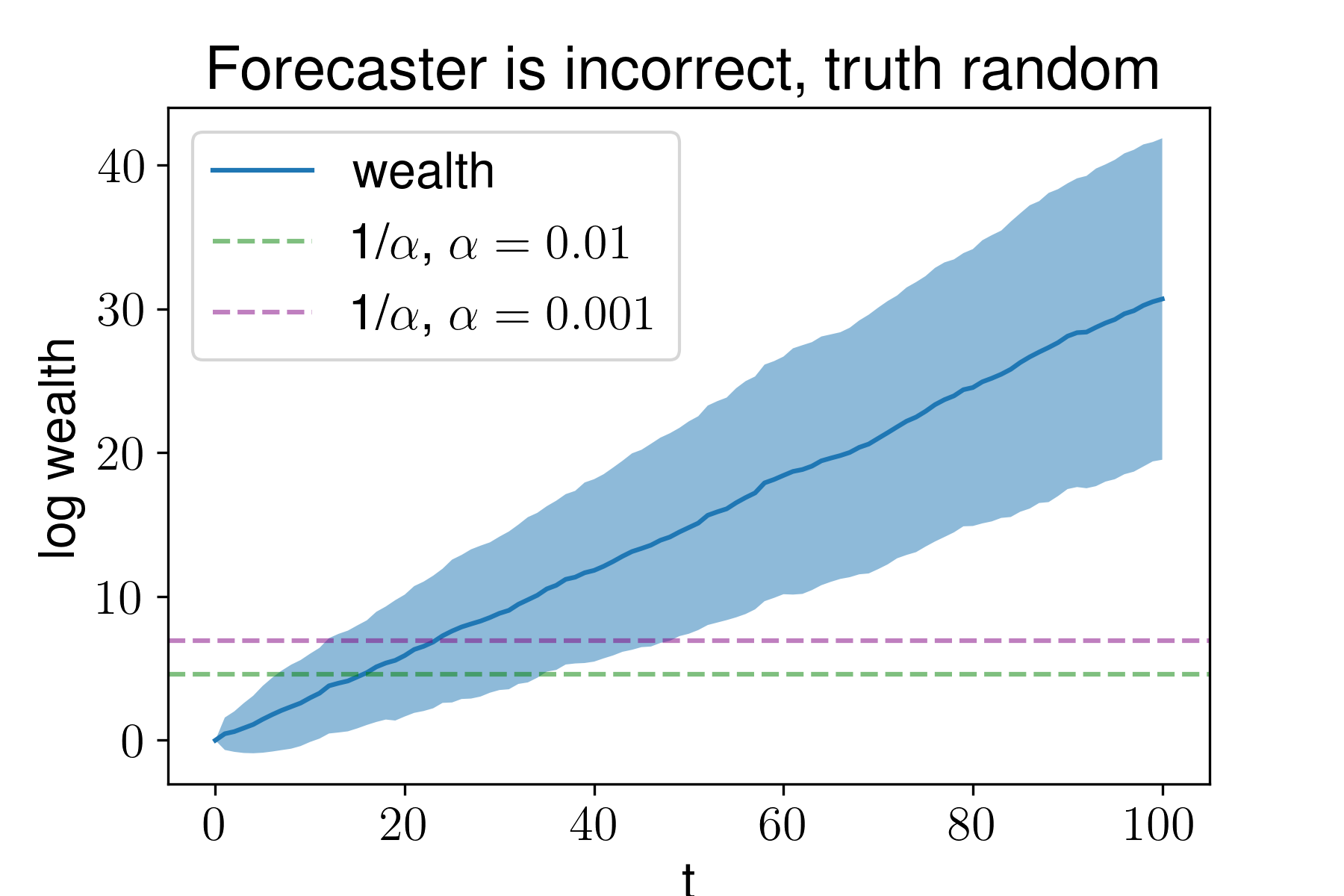
Average wealth is given by the dark blue line, and the shaded area is the standard deviation from 100 trials. The horizontal lines give the wealth that we need to acquire to reject the accuracy of the forecaster at the desired confidence level.
Note that y-axis is the log wealth, not the wealth. So here we would reject that the forecaster is accurate within roughly 20 trials at both \(\alpha=0.01\) and \(\alpha = 0.001\).
Perhaps it’s unreasonable for the forecaster to be entirely decoupled from reality. Here’s what happens if the forecaster is incorrect, but \(P_t\) is correlated with the truth. More precisely, we let \(p_t = \xi_t + N(0,1)\). That is, the forecaster uses a noisy version of the parameter used to generate reality.
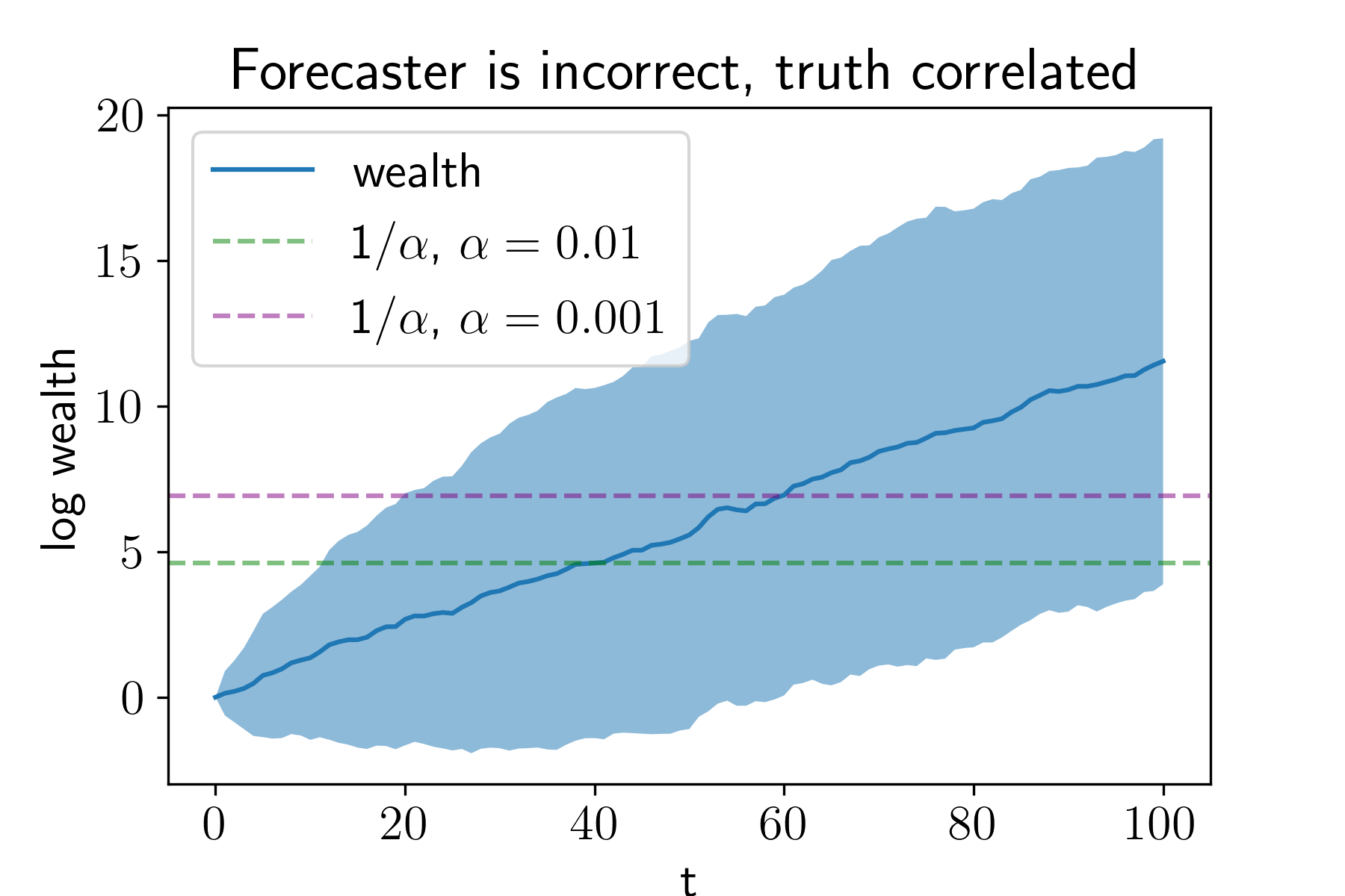
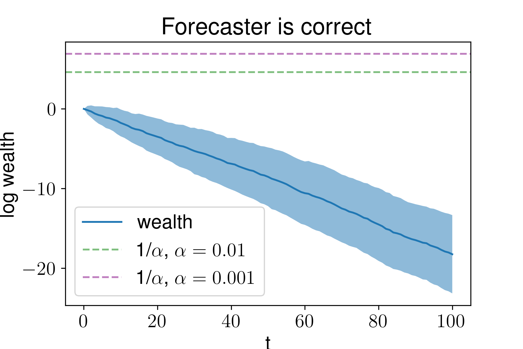
Here we still make money against the forecaster, but more slowly. It takes roughly 40 trials to reject at \(\alpha = 0.01\) and roughly 60 at \(\alpha = 0.001\). Finally, to make ourselves feel better, let’s make sure that we don’t make money against a forecaster who knows the truth, i.e., \(p_t= \xi_t\). Here our wealth decreases over time:
In these experiments the forecaster specifies their prediction and we receive the feedback immediately. But this need not be the case; we could make many bets against the forecaster at once and wait for them to resolve.
This isn’t the end of the story. One could imagine doing a more detailed empirical and theoretical analysis of precisely which betting strategies are best against which kinds of forecasters (for instance, if you suspect a forecaster is predisposed to be biased towards certain events, how should you bet?) or understanding when various betting strategies will fail. But I think this could be an interesting way to test real-world forecasters (eg political pundits or superforecasters).
Back to all notes


